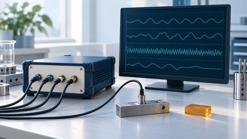
A trustworthy measurement log lets another engineer reconstruct what was measured, when it was acquired, and how the saved numbers were produced. Start with a channel dictionary and a timing definition, then prove that the saved file survives a complete test and read-back. A moving trace on a screen establishes only that some values are reaching the display.
Define the record before choosing software
Write down the decision the test must support: a steady-state temperature, a transient peak, or the relationship between two signals. That decision determines the needed bandwidth, sample rate, synchronization and uncertainty. Select compatible sensors and acquisition hardware with the responsible measurement engineer; logging software cannot recover a signal that the measurement chain failed to capture.
Give every channel a stable identifier. Record the physical input, sensor serial number, engineering units, calibration reference, range, scaling and relevant machine state. Keep the acquisition configuration with the data, including changes made between runs. A column headed “Input 1” becomes difficult to interpret when a cable is moved.
For one concrete file-format example, NI documents TDMS file, group and channel properties, including waveform start time and time increment. Whatever format you choose, test whether your export retains equivalent context. A plain numeric export may need a separate metadata file.
Separate sample timing from file-writing time
Identify the event represented by each timestamp. It might be the hardware acquisition start, the arrival of a block at the computer, or the moment a row is written. For uniformly sampled data, a start time, verified interval and sample index can define the time axis. For irregular acquisition, retain the actual timing information and its uncertainty.
NI's DAQmx timing documentation distinguishes hardware sample-clock configuration from reading acquired data. Reading 1,000 samples at a time changes the transfer block; it does not by itself establish the sample rate. For multiple devices, document their clock and trigger relationship and verify the alignment needed for the decision.
On a narrow screen, scroll the table horizontally. Keyboard users can focus it and use the arrow keys.
| Record element | What to preserve | Verification |
|---|---|---|
| Channel meaning | Input, sensor, unit, scaling, calibration | Apply an appropriate known input and check saved values |
| Time axis | Clock, trigger, interval, time zone, index | Compare expected duration and count; investigate discontinuities |
| Data integrity | Errors, dropped blocks, overflow and stop reason | Read the file back and reconcile all channels |
| Reproducibility | Configuration, software version, raw/derived distinction | Recreate one reported result from preserved raw data |
Commission the complete logging path
- Run a short known-input trial. Inspect values, units, channel order, polarity and timestamps in the saved file.
- Run long enough to exercise normal file rollover and storage behavior. Record stop/restart boundaries and whether new files preserve their sequence.
- In a controlled test environment, check how a disconnected sensor or interrupted acquisition is represented. Retain fault flags alongside values.
- Open the result using the intended downstream reader. Compare sample counts, metadata and representative raw values with the acquisition record.
Preserve the raw file as the reference. Store filtering, resampling and unit conversion as documented derived work. If a reviewer needs a spreadsheet, supply a manageable extract with explicit units and a link to the full record. Keep the original precision even when the report displays rounded values.
Worked example: locate a missing interval
Fictional acquisition: two channels run at 100 samples/s/channel for a 60-second acquisition window. Each should contain 6,000 samples. Zero-based indices run from 0 through 5,999.
One channel jumps from index 2,999 to 3,100. The missing indices, 3,000 through 3,099, contain 100 scheduled samples: 100 ÷ 100 = 1 second of missing samples. With no other losses, that channel contains 5,900 samples.
Mark the interval and determine whether it invalidates the intended result. A peak could have occurred during the gap. Interpolation may support a clearly labeled visualization, but an acceptance result needs an explicit treatment of missing evidence.
For vibration-specific choices about mounting, conditioning and bandwidth, continue with making vibration measurements comparable.
Use the working record
Download the editable measurement log record. Save a copy, complete the actual requirements and evidence fields, and review open issues with the responsible owner. The plain-text record includes instructions, units where needed, the fictional example, and source references.