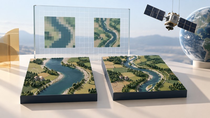
Satellite imagery becomes useful when a question determines the data you choose. Looking for seasonal vegetation change, a broad reservoir shoreline or regional development calls for different observations. Begin with a defined area and time window, then select a sensor and processing level that can show the feature at the scale you need.
Turn the question into an observation plan
Write the place, feature, date range and smallest change you want to distinguish. For example: “Compare the visible shoreline of this reservoir in late summer across two years.” That is more testable than “Find a recent satellite photo.” Keep the same area of interest for both dates and note the coordinate system used for measurements.
Pixel size sets a sampling scale. A 10-meter pixel covers 100 square meters on the ground; a narrow object can occupy only part of it. Zooming or resampling makes a picture larger without adding new observations. Feature recognition also depends on contrast, optics, processing and surrounding land cover.
Choose a public source that fits
Scroll the table horizontally on small screens. Keyboard users can focus the table region and use the arrow keys.
| Source | Useful starting task | Check before comparing |
|---|---|---|
| Copernicus Sentinel-2 | Vegetation, land cover, broad shorelines and other optical surface features. | Band resolution, acquisition time, clouds and processing level. |
| USGS Landsat archive | Consistent regional observations and longer historical comparisons. | Sensor, product collection, quality flags and reflectance scaling. |
| Radar products | Questions where cloud cover limits optical observations. | Viewing geometry, polarization, terrain effects and processing; interpretation needs a radar-specific method. |
Copernicus documents Sentinel-2 with bands sampled at 10, 20 and 60 meters, and Level-2A products providing atmospherically corrected surface reflectance. Native resolution therefore varies among bands within one mission. Choose the required bands before deciding that a feature can be measured.
Start in Copernicus Browser for Sentinel data or USGS EarthExplorer for Landsat searches. Interactive access and downloads may require an account. USGS explains surface reflectance as a product intended to reduce atmospheric influences for surface comparisons; residual clouds, shadows and other artifacts still need attention.
A repeatable optical-image workflow
- Find the location and draw or save the area of interest.
- Select the mission and product level, then search a time window around the event or season of interest.
- Use cloud filters to narrow candidates, then inspect clouds and shadows over the actual study area. A scene-wide percentage can hide a cloud directly over your site.
- Select two images with comparable season, illumination and processing. Record both acquisition times, sensor identifiers and product IDs.
- Use the same band combination, display stretch and viewing extent. Compare natural-color views first, then use a justified false-color or index view.
- Save the product metadata and quality information with the image. Separate a display export from the numerical source data.
For measurements, use a GIS workflow with suitable coordinates and pixel alignment. A web-browser screenshot is useful for discussion; numerical analysis also needs the source data and processing metadata.
Worked example: interpreting a shoreline change
Use “observed difference,” “possible explanation” and “evidence needed” as separate fields in your notes. This keeps a visually persuasive comparison from becoming an unsupported causal claim.
Keep numerical processing traceable
An index such as NDVI combines near-infrared and red reflectance: (NIR − red) ÷ (NIR + red). For invented reflectances of 0.50 and 0.20, NDVI is approximately 0.429. This illustrates the calculation; it is neither a crop diagnosis nor a universal health threshold.
Use the product's specified scale factors, offsets and quality masks before calculating. USGS's Level-2 scaling instructions distinguish stored integers from physical values. A rule copied from a different sensor or product generation can alter the result. Exclude invalid pixels and handle a zero denominator explicitly.
Keep the original product IDs, bands, masks, scaling, projection and software steps. Avoid mixing a contrast-enhanced display image with physical reflectance data. For cross-sensor work, establish comparability rather than assuming identically named bands have identical responses.
Save a comparison someone else can check
Download the imagery comparison record. It includes a place for acquisition dates, product IDs, processing choices and alternative explanations. Add a source link and the relevant attribution or license when exporting imagery.
Revisit the result if a replacement product is issued, the quality mask changes, or a new observation contradicts the apparent trend. For the spacecraft tradeoffs behind these observations, see small satellites and mission design.
Sources and further reading
Source links reviewed September 28, 2026. Check current service terms, equipment documents and operational notices when applying the guide.