An AI model estimates that a crop is close to needing water. Is it close enough to start the pump? In a field test on maize and soybean, the model predicted soil-water depletion with errors measured in tens of millimeters. Whether a grower can act on that prediction depends on how far the block is from its irrigation trigger and what the soil shows today.
How an irrigation model learns soil-water depletion
Precious Amori and colleagues used data from 2020 and 2023 to train several models on maize and soybean. The inputs brought together weather, soil properties, remote observations and management history. The target was soil-water depletion, the depth of water missing from the crop’s root zone relative to field capacity. Their best performer on an independent 2024 season was extreme gradient boosting, which builds a sequence of decision trees, each helping correct earlier prediction errors. Amori and colleagues’ field deployment and validation study.

In 2024 the model’s root-mean-square error was 22 mm for maize and 24 mm for soybean. This statistic summarizes errors across observations and gives larger misses more weight. The model generalized less well to a separate 2021 dataset. Agreement between a model and another irrigation scheduler is a useful cross-check. To find out how much water a farm actually saves, a trial also needs metered applications and a harvest comparison.
Ground-check the model at the right depth
To test a prediction, match its date, depth and location with the observations. Begin with a unit the farm can water independently. Record the crop, growth stage, active rooting depth, soil layers and time of the last rain or irrigation. A seedling and an established crop can use different depths of the same soil. Compare measurements within each management zone before averaging across fields. The field-scouting example explains why a delivery fault deserves its own check.

Field capacity describes how much water the soil retains after excess water has drained. The permanent wilting point is the lower reference used in estimating plant-available water. Their difference, multiplied by the thickness of a soil layer, gives that layer’s available water capacity. The difference between field capacity and the current water content gives its depletion. Add the layers inside the active root zone. Local soil values, crop stage and the irrigation system determine the depletion that should trigger action. Minnesota Extension on sensors, soil water and placement.
Can an independent water budget reproduce the model’s call?
Return to the fictional block where the model reported 35 mm. Two days earlier the grower took soil readings. The block has an effective root depth of 600 mm at the current crop stage. It has two 300 mm layers. The moisture readings are volumetric fractions, so 0.25 means water occupies one quarter of the measured soil volume. The example uses millimeters of water depth throughout. Its soil values and trigger are teaching assumptions.
- Upper layer. Field capacity is 0.30 and current water content is 0.25. The depletion is (0.30 − 0.25) × 300 mm = 15 mm.
- Lower layer. Field capacity is 0.29 and current water content is 0.25. The depletion is (0.29 − 0.25) × 300 mm = 12 mm.
- Starting balance. The measured root zone is 27 mm below field capacity. Suppose the available fraction between field capacity and wilting point is 0.14 in each layer. Total available water is 0.14 × 600 = 84 mm. A locally chosen trigger of 40% depletion would be 33.6 mm.

Carry the balance forward from the measurement time. Add estimated crop evapotranspiration (ET), subtract rain retained in the root zone, and subtract net irrigation retained there. Reference ET from a weather station describes a reference surface. When using a crop-coefficient method, use the coefficient appropriate to the crop and growth stage to estimate crop ET. We assume negligible groundwater contribution in this example. Runoff and drainage beyond the roots do not refill the active zone. Start a new balance when a field measurement establishes a better starting point. Extension’s irrigation checkbook method.
Account for the time the system needs to reach the block, any change in rooting depth and the lead time of the rain forecast. If the readings already include yesterday’s rain, enter only events since those readings. The satellite ET guide explains why a monthly map alone cannot settle a daily schedule.
After accepting a recommendation, measure what the system delivers
Suppose the dry scenario occurs and a field check supports the 35 mm deficit. For this example the grower wants to leave 15 mm of storage below field capacity. That means adding 20 mm net. If the estimated application efficiency for this irrigation is 0.80, the gross depth is 20 ÷ 0.80 = 25 mm. Across one hectare, 25 mm is 250 cubic meters at the point where gross delivery is measured. A different area, wetted pattern or efficiency estimate changes the result.

Check the block area, meter volume and operating flow before converting a depth to runtime. After the run, compare timed emitter output across the block. Recheck moisture at the relevant depths after redistribution. If the inlet meter shows the planned volume but one end stays dry, turn back to delivery uniformity. Extending the whole run can push water below the roots in the wetter rows.
Download the field water record for checking a prediction (Markdown) to keep soil layers, observed rain, forecast scenarios, meter totals and the next field check together.
Illustrated field notes
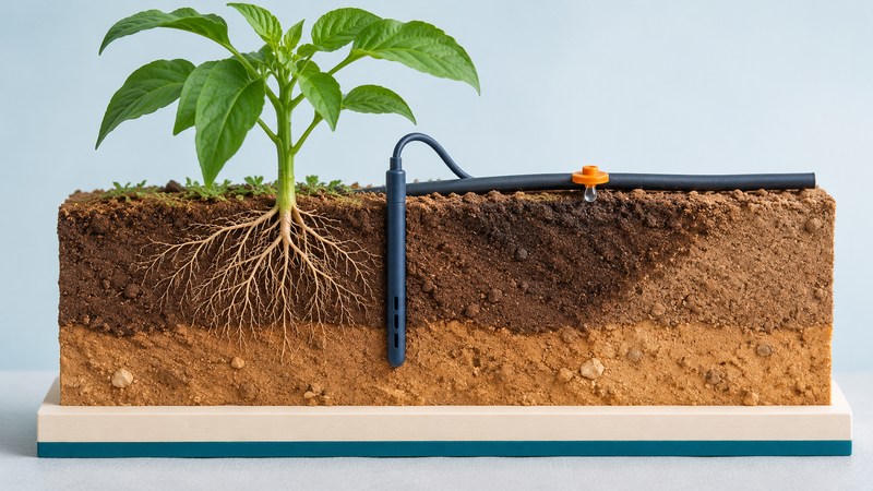
These conceptual illustrations show the other evidence a scheduler may use. Open a subject for the large images.
Weather, remote observations and drought


Automation, connectivity and thresholds


Costs, previous seasons and shared records


