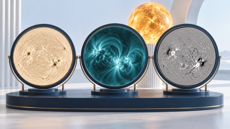
Solar Dynamics Observatory images let you compare the Sun's visible surface, magnetic patterns and hot atmosphere. Begin with the product label and timestamp. A bright patch in an ultraviolet image, a dark sunspot and a black-and-white magnetic patch describe different measurements, even when they occupy the same solar region.
Choose a product for your question
Open the SDO image page. The Atmospheric Imaging Assembly (AIA) provides images in selected wavelength bands. The Helioseismic and Magnetic Imager (HMI) derives surface intensity, velocity and magnetic measurements. The Extreme Ultraviolet Variability Experiment (EVE) studies the Sun's spectral irradiance, adding a whole-Sun perspective.
| Product | Useful first question | Read it with this context |
|---|---|---|
| HMI continuum intensity | Where are sunspots on the visible surface? | Display processing can flatten the brightness difference between center and limb. |
| HMI magnetogram | Where are opposite magnetic polarities? | Check whether it is line-of-sight or vector data and read its polarity convention. |
| AIA 171 Å | What loop structures appear in the quiet corona? | This band emphasizes particular ion emission and temperature response. |
| AIA 193 Å | How do coronal bright regions and dark areas compare? | Response includes coronal material and much hotter flare plasma. |
| AIA 304 Å | Where are structures in the chromosphere and transition region? | Helium emission highlights a different component from the iron-dominated coronal bands. |
The team's channel reference gives the spectral bands, principal ions and typical temperature responses. Å means angstrom: 10 Å = 1 nanometer, so 171 Å = 17.1 nm. The familiar display colors are assigned to these otherwise invisible wavelengths.
Check the clock before comparing the Sun
Read the time embedded in each image and retain the stated time standard. Two panels on a “latest” page may have different acquisition times. A delayed image can be scientifically useful, but it should be described by its actual timestamp.
SDO's browse-data guidance describes near-real-time images updated about every 15 minutes. That public update interval differs from the instrument's acquisition cadence and from the frame spacing of a particular movie. For older observations, use the dated browse archive linked from the data page.
If an image appears frozen or a movie jumps, inspect the times and check the mission's notices. Gaps can come from observing interruptions, processing or delivery. A missing frame carries no evidence that a solar feature vanished.
A repeatable ten-minute image exercise
- Choose an available UTC time and open an HMI continuum image plus AIA 171 and 193 images as close to that time as practical.
- Record each product, resolution and timestamp. Keep the time differences visible in your notes.
- Pick one region away from the limb. Note its position relative to the disk center and save the source URLs.
- Describe what is directly visible in each product: a dark patch, a loop, a brightening or a diffuse region.
- Open a short movie in one channel. Compare several frames with their timestamps, keeping the scale and orientation consistent.
- Write an interpretation separately from the observations and name one additional measurement that would test it.
Interpret brightness, motion and overlays carefully
AIA bands have temperature responses, but a single displayed pixel is not a thermometer. Emission along the line of sight, material density, instrument response and image scaling contribute to brightness. Quantitative temperature analysis combines calibrated channels with an explicit method.
A feature moving across the disk over days may reflect solar rotation. Motion near the limb is foreshortened, and an expanding structure seen in projection requires geometry before you can infer its true speed. First record the elapsed time and image scale; keep apparent motion separate from a physical velocity.
Some SDO products include PFSS magnetic-field overlays. These are model-based field traces, distinguishable from the observed image underneath. NASA CCMC explains the assumptions behind the PFSS coronal-field model. Keep the product label when sharing them. For the broader issue of translating invisible wavelengths into pictures, see reading Webb images.
Use forecasts for Earth-impact questions
A solar image provides context for activity. A prediction of effects at Earth additionally needs information about eruptions, particle transport and the solar wind. For operational expectations, consult NOAA's three-day space-weather forecast, checking its issue time, valid period and separate categories for geomagnetic activity, radiation storms and radio blackouts.
Download the SDO comparison log and open it in a text editor. It preserves the product labels, time offsets, direct observations, interpretation and forecast context. The exercise uses online images; direct solar viewing requires specialized equipment and appropriate solar viewing precautions.