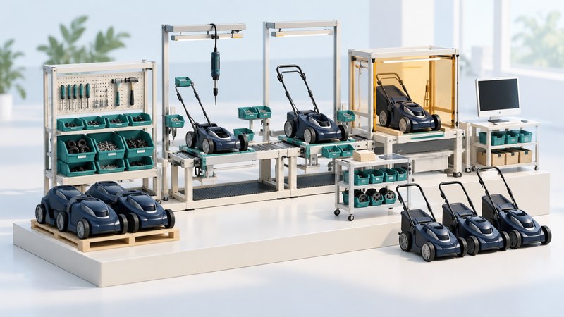
ROMEtex was described in March 2001 as a virtual lawnmower factory for the Institute of Operations Management’s Remote Operations Management Education project, or ROME. Its subject was learning how a factory works: the flow of materials, production decisions, and opportunities for improvement.
What the 2001 training concept proposed
The contemporary announcement described a PC/web-based learning package in which participants could explore a simulated manufacture-and-assembly business and follow links into a handbook. The proposed factory problems connected to production, inventory, performance, and the Institute’s operations-management syllabus. The factory was presented as nearing completion at the time.
That account establishes the announced teaching concept. It does not establish a subsequent launch date, measured learning results, or present-day availability. Treat ROMEtex as a historical example of workplace learning through a simulated business. The explanation below explores the ideas with an original fictional exercise; it does not reproduce the software or its exercises.
Why use a mower factory to teach operations?
A mower makes a useful teaching object because it can be represented as a small sequence of parts and assemblies. A simple model can ask whether components arrive when needed, where unfinished work waits, and whether improving one workstation increases completed output. Learners can make a decision, observe the modeled consequence, and explain the tradeoff.
NIST’s research on discrete-event simulation of factory operations describes using models to examine throughput, capacity, and bottlenecks under different scenarios. Those are useful analytical ideas for this exercise; the NIST research is separate from the ROMEtex project.
| Question | What a learner would record |
|---|---|
| Are materials available? | Component requirements, supply timing, shortages, and assumptions about replenishment. |
| Where does work wait? | Queue size before each station and how it changes through the modeled period. |
| What limits output? | Processing capacity, interruptions, rework, and dependencies between stations. |
| Did the change help? | Completed units, time in the system, work in progress, and the cost or resource change. |
A fictional three-station assembly exercise
Assume three independent stations in sequence, one mower processed at a time per station, unlimited material supply and intermediate waiting space, and no breakdowns, scrap, changeovers, or transfer time. Consider steady operation after startup. These simplifying assumptions make the arithmetic visible; they are not factory measurements.
| Station | Minutes per mower | Capacity per hour |
|---|---|---|
| Prepare chassis | 6 | 60 ÷ 6 = 10 |
| Fit components | 10 | 60 ÷ 10 = 6 |
| Final check | 5 | 60 ÷ 5 = 12 |
The component-fitting station limits ideal steady output to 6 mowers per hour. If chassis preparation continuously releases 10 per hour while fitting accepts 6, the waiting inventory before fitting grows by 4 per hour under these assumptions. Making the final check faster does not remove that bottleneck.
Now suppose an independently justified change reduces fitting time to 7.5 minutes. Its ideal capacity becomes 8 per hour; the line’s ideal upper rate becomes 8 per hour, with fitting still the slowest station. Chassis preparation would still outpace fitting by 2 per hour if allowed to run continuously. Coordinating releases can therefore matter as well as increasing capacity.
These rates describe capacity after startup, not an exact first-hour shipment count. The first mower must pass through all three stations. Real results also depend on failures, staffing, variable times, and quality. Record those assumptions before treating a model as a forecast.
Turn the example into a learning exercise
- State a question, such as whether a faster inspection station would improve completed output.
- Write the process sequence and record the inputs, units, and assumptions.
- Calculate a baseline and explain which station limits the ideal rate.
- Change one input, calculate again, and record both the benefit and the remaining constraint.
- Add a realistic complication, such as a limited buffer or downtime, and explain why a simple capacity calculation is now insufficient.
A useful classroom discussion asks learners to defend their assumptions and identify the evidence needed from an actual factory. NIST’s Simantha manufacturing-simulation resource illustrates how a more detailed model can represent machines, finite buffers, and maintenance. It is a separate simulation resource, not a replacement or continuation of ROMEtex.
The durable lesson is to connect a proposed improvement to the whole process and to state what the model can support. A visually convincing factory scene is only the interface; the assumptions and checks determine whether its results are useful.