
An RFID read map helps a team see where a defined test succeeded or failed. Its value comes from known test positions, repeatable observation windows and visible denominators. A smooth colored surface can hide gaps in evidence unless those details travel with it.
Use this guide after establishing compatible tags and readers and a controlled test plan. It shows an invented stationary grid experiment, not a performance claim for any product. A moving-cart or handheld-count workflow requires its own representative trials.
Define what one colored cell means
Choose a physical coordinate origin, units, tag height and orientation. Mark the intended reading area and identify any deliberately placed tags outside it. At each point, run a fixed observation window with the same configuration and reset conditions. Define success before collecting data: for example, the expected target identity appears at least once during that window.
Count each trial once for target success. Repeated reports of the same target inside the window do not create more successful trials. Independently record whether any known out-of-zone test tag appeared. This gives two measures: target success and trials with an unwanted read. A run can have both.
Save reader and antenna identities, firmware, region/profile, settings, target construction, object surface and timestamp context with the dataset. Include a reason when a scheduled point is untested. A zero-success test and an absent test have different meanings.
Read a complete worked example
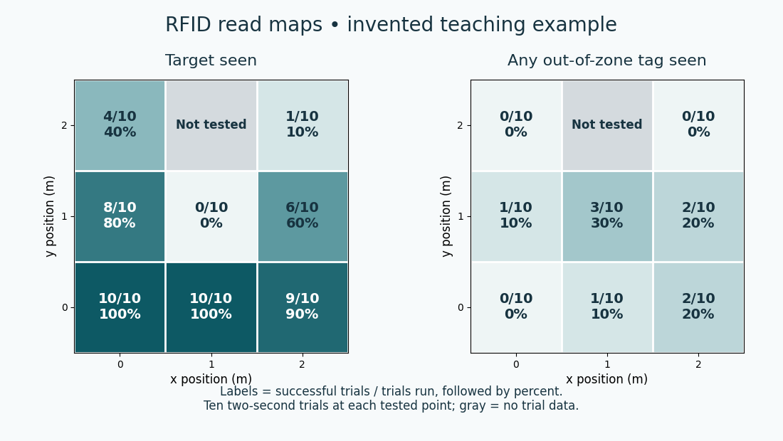
The invented experiment uses a three-by-three grid at x and y coordinates 0, 1 and 2 metres. Each tested point has ten two-second trials, with one intended target at that point and known out-of-zone tags kept fixed. The point (1, 2) was not tested because access was blocked. The sample is deliberately small to make the arithmetic easy to inspect.
On a small screen, scroll sideways to read all columns.
| Position (x, y), m | Trials | Target success | Any unwanted read |
|---|---|---|---|
| (0, 0) | 10 | 10/10 (100%) | 0/10 (0%) |
| (1, 0) | 10 | 10/10 (100%) | 1/10 (10%) |
| (2, 0) | 10 | 9/10 (90%) | 2/10 (20%) |
| (0, 1) | 10 | 8/10 (80%) | 1/10 (10%) |
| (1, 1) | 10 | 0/10 (0%) | 3/10 (30%) |
| (2, 1) | 10 | 6/10 (60%) | 2/10 (20%) |
| (0, 2) | 10 | 4/10 (40%) | 0/10 (0%) |
| (1, 2) | 0 | Not tested | Not tested |
| (2, 2) | 10 | 1/10 (10%) | 0/10 (0%) |
Across tested positions there are 48 target successes in 80 trials: 60%. Nine of those 80 trials contain an unwanted read: 11.25%. These summarize this chosen grid and trial allocation. They are not a forecast for an operating site or evidence about the untested point.
The center point was tested and failed every target trial, so it merits investigation. The gray point needs a test before drawing a conclusion. At (2, 0), target capture is high but unwanted reads still occur. Reporting only the target map would conceal that tradeoff.
Keep signal measurements alongside outcomes
Reader telemetry can help diagnose a pattern. Zebra's MAUI Android SDK guide, for example, describes configurable reports containing antenna identity, channel, peak RSSI, phase, seen count and timestamps. The fields actually returned depend on the reporting configuration. Check field availability, units, aggregation and time basis for the installed reader and SDK before combining exports.
RSSI is a received-signal metric; converting it into distance requires an appropriate, validated model and conditions. The map here uses positions established by the test setup, not coordinates inferred from RSSI. Label a measured signal map with the actual metric and units. Keep missing telemetry separate from measured zero values.
When several antennas report one target, preserve their identifiers. Combining them can answer whether the system captured the item; separating them can explain which antenna contributed. Decide which question each plot answers and state the aggregation.
Compare changes without changing the question
Change one relevant factor, such as tag placement, and repeat the same positions and trial windows. Keep the same color limits on before-and-after plots and show both success and unwanted-read maps. A map that rescales itself can make a weak result look visually strong.
Retain failed runs, test order and environmental changes. Add repetitions and representative movement tests according to the decision being made. Ten trials at a point are a teaching example, not a universal acceptance sample. Avoid interpolating a success region across untested positions unless the model and its uncertainty are separately justified.
For operating acceptance, connect the radio results to the task: correct basket, correct passage or completed count. The RFID test-plan guide covers controlled comparisons, and the portal guide adds passage boundaries and direction.
Reuse the example with its definitions
Download the invented summary CSV and invented per-trial CSV. The summary includes coordinates, trials, successes, unwanted-read trials and a note for the missing point. The trial file lets you independently reconstruct all counts. The data dictionary and instructions define fields, units and calculation rules.
When replacing the sample with field results, retain the metadata and expected-tag definitions in a separate controlled record. Mark the resulting plot with the tested configuration, observation window, date and limitations. A useful map should let a colleague trace every colored cell back to its evidence.
Keep a working record
Download the editable working record (plain text). It includes purpose, instructions, evidence fields and this guide's source links. Save a separate copy for each evaluation and record unresolved issues with their owner.
Related reading
Researched and updated September 20, 2026. Recheck source documents when equipment, software or applicable requirements change.